When Kalshi and Fed funds futures disagree

Can't find what you need? Get in touch

And why prediction markets data is now a must-have for macro rates traders

By Etienne Mercuriali, Director of Research at BMLL.

Supporting research by Ben Bingham, BMLL.

1 October 2026

Prediction markets have grown exponentially over the past year and provide potential new sources of alpha for systematic and macro trading decisions. A critical driver for macro trading is changes in US Fed Rates, which have historically been hedged using 30-Day Federal Funds futures on the CME. By comparing Kalshi’s Fed decision prediction markets against this futures contract, we can see how the two instruments compare and what additional information is contained in Kalshi data.

Using BMLL's normalised market data for both instruments, we see that Kalshi priced less tightening by the Fed than the CME Fed Funds future in the month before both the July and September 2026 decisions (median gap 2.9 basis points in July and 1.7 in September), whilst the CME future reacted first on economic announcements, such as the Consumer Price Index (CPI) on 11 September 2026.

The differences between these two markets allow us to test simple cross-market trading strategies. We show that a hedged position across both markets, held until the Fed rate announcement, could have achieved a positive P&L for both the July and September 2026 decisions.

For anyone looking to hedge or trade based on the Fed rate, prediction markets are therefore an important dataset.

Prediction markets price different, growing and tradeable views from traditional markets

US Fed rates are a major factor for many macro traders. Set by the Federal Open Market Committee (FOMC) several times per year, predicting and hedging potential rate changes is a significant and important part of a trader’s workflow.

Historically, hedging the Fed rates has been achieved through 30-Day Federal Funds futures (ZQ or FFF), a future listed on the CME and which settles against the monthly average Effective Federal Funds rate. However, prediction markets now offer a potential alternative. For example, Kalshi’s KXFEDDECISION market instead divides the meeting into five mutually exclusive outcomes: a hike greater than 25bp, a 25bp hike, no change, a 25bp cut, or a larger cut. Understanding how these products behave is critical for market participants – macro traders can ensure that they optimally hedge, whilst speculators can potentially exploit market inefficiencies between the products to find new sources of alpha.

Using BMLL data, we analyse both the CME Fed Future and Kalshi prediction markets, finding several important results:

Ahead of the 12 FOMC meetings from May 2025 to September 2026, Kalshi and the CME futures held differing views of the coming Fed decision, by up to 2.8 basis points.
Following the CPI data release on 11 September, the CME futures moved first, about 0.6 seconds ahead of the Kalshi market.
The Fed decision itself closed most of the gap in July and September. Twenty minutes after the announcement, the futures-implied decision sat 0.52bp from the outcome in July and 0.75bp in September. June, when Kalshi priced a hold with near certainty, stayed 1.61bp away.

Turnover on Kalshi continues to grow, although displayed depth remains far below that of the futures. Anyone trading these markets will need to monitor this, extend the cross-market relative value analysis to other contracts and markets, and re-run it over time.

We then build a toy trading strategy to test whether these differences could have been traded. It made a modelled net profit of US$3,944 in the July FOMC meeting and US$791 in September. Two meetings are a small sample, but they suggest that prediction market data deserves a place in a Fed rates workflow.

One policy decision, two different markets

The FOMC sets a target range for the federal funds rate. CME’s 30-Day Federal Funds futures (ticker ZQ, or FFF for short) settle against the monthly average Effective Federal Funds rate (EFFR) and are priced as 100 - EFFR. Kalshi’s KXFEDDECISION market instead divides the meeting into five mutually exclusive outcomes: a hike greater than 25bp, a 25bp hike, no change, a 25bp cut, or a larger cut, with binary payouts based on the outcome.

That distinction presents a challenge when trying to compare the two markets. A Kalshi contract maps directly to a meeting outcome. ZQ (Fed Funds Futures) embed a month of EFFR that happens to contain the decision and can also contain exposure to another meeting or other factors. Therefore, whilst the prices are related, they are not identical.

To account for this, we put both markets on a common basis-point (DV01) scale. Kalshi’s five prices are normalised into an expected decision. The futures strip is decomposed into calendar-weighted policy jumps using the commonly accepted method popular with macro traders and popularised by CME. The comparison throughout the article is the futures-implied decision probability in basis points minus the Kalshi-implied decision: a positive number means the futures model prices more tightening of the Fed rate.

A roughly 2bp fair-value disagreement persisted for a month before the July and September 2026 Fed decisions

Once we model the decision probabilities exhibited by both markets, the differences between the two fair values, implied by Kalshi traders on one side and by CME on the other, become clear. Ten days before the FOMC, the gap was 2.7 basis points (bp) in July and 1.7bp in September 2026. Earlier meetings show no consistent sign (Figure 1). In September 2025, for example, Kalshi priced a higher rate than the futures, by 1.94bp ten days out. Kalshi quote data starts in April 2026; for earlier meetings the Kalshi value comes from a 60-minute volume-weighted average of trade prices, so the earlier rows are less comparable.

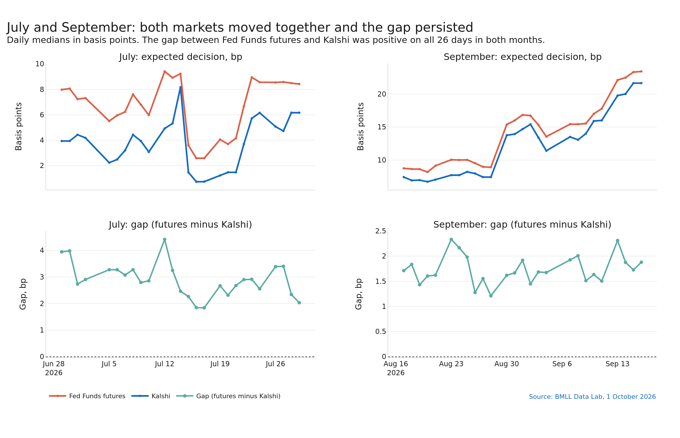
In the most recent months, Kalshi consistently predicted more easing (or less tightening) than the futures, as shown in Figure 1. In July the difference between CME and Kalshi was positive on every one of 26 days, ranging from 1.8bp to 4.4bp (median 2.88bp). Ten minutes before the 29 July announcement, the futures model implied +7.3bp against Kalshi’s +4.7bp. The FOMC left rates unchanged, so Kalshi’s implied prediction was closer to the realised decision at that instant. In September the opposite was true: the FOMC raised the target range by 25bp, making the futures the closer estimate. The September gap was also positive on all 26 days, ranging from 1.2bp to 2.3bp (median 1.68bp).

Whilst the implied fair value differs between contracts, changes in value are clearly correlated, as shown in Figure 2, suggesting that both contracts react to news and events ahead of FOMC announcements. In September both markets repriced by about 15bp over the month while the gap stayed between 1.2bp and 2.3bp.

Once the FOMC decisions were made, the gap between the two markets largely closed. Kalshi resolves mechanically to the Fed decision. The futures converge as well, but not fully: they settle on the average EFFR for the rest of the month, which also reflects other information. To measure this, we freeze the futures-implied decision 10 minutes before the announcement and add only the observed price move in the hedging contracts. Twenty minutes after the announcement, that estimate sat 0.52bp from the decision in July (rates unchanged) and 0.75bp from it in September (25bp hike). June, when Kalshi priced a hold with near certainty, sat 1.61bp away. Figure 3 shows the three meetings.

Fig 1: Expected decision implied by Fed Funds futures minus that implied by Kalshi, 12 meetings and five horizons (bp). Positive = futures price more tightening.

Fig 2: July and September 2026 expected-decision paths and daily gap between Fed Funds futures and Kalshi (bp).

Fig 3: Expected decision around the June, July and September 2026 FOMC announcements. Dotted: futures estimate frozen 10 minutes before the announcement plus the later price move.

Fed Funds futures moved first around the September 2026 CPI announcement

The 11 September 2026 CPI release allows us to answer another question: how quickly both products react to news and economic announcements.

Following the CPI data release, where inflation exceeded expectations and increased the likelihood of a rate increase, the Fed Funds futures hedge (October and November contracts) first moved towards a higher rate 1.2 seconds after the release, following a brief move the other way. Kalshi’s repricing, mapped to basis points from the 25bp-hike outcome, first moved 1.8 seconds after the release, 0.6 seconds later. The lag grew with the size of the move: the futures had repriced by 1bp after 1.3 seconds and by 2bp after 2.3 seconds, against 4.9 and 10.4 seconds on Kalshi. By 30 seconds both markets had repriced by about 4.9bp.

Liquidity in order books tends to reduce significantly before economic releases, as market makers move away due to the uncertainty of the announcement. As you can see in Figure 4, order book depth on both Kalshi and CME significantly reduced ahead of the CPI release. Interestingly, the futures order book depth recovers significantly quicker. This could be due to the nature of market maker behaviour on the two venues, or due to the differences between the contract specifications.

Fig 4: CPI reaction and book replenishment for Fed Funds futures and Kalshi Fed decision markets

Liquidity in Kalshi Fed predictions is growing

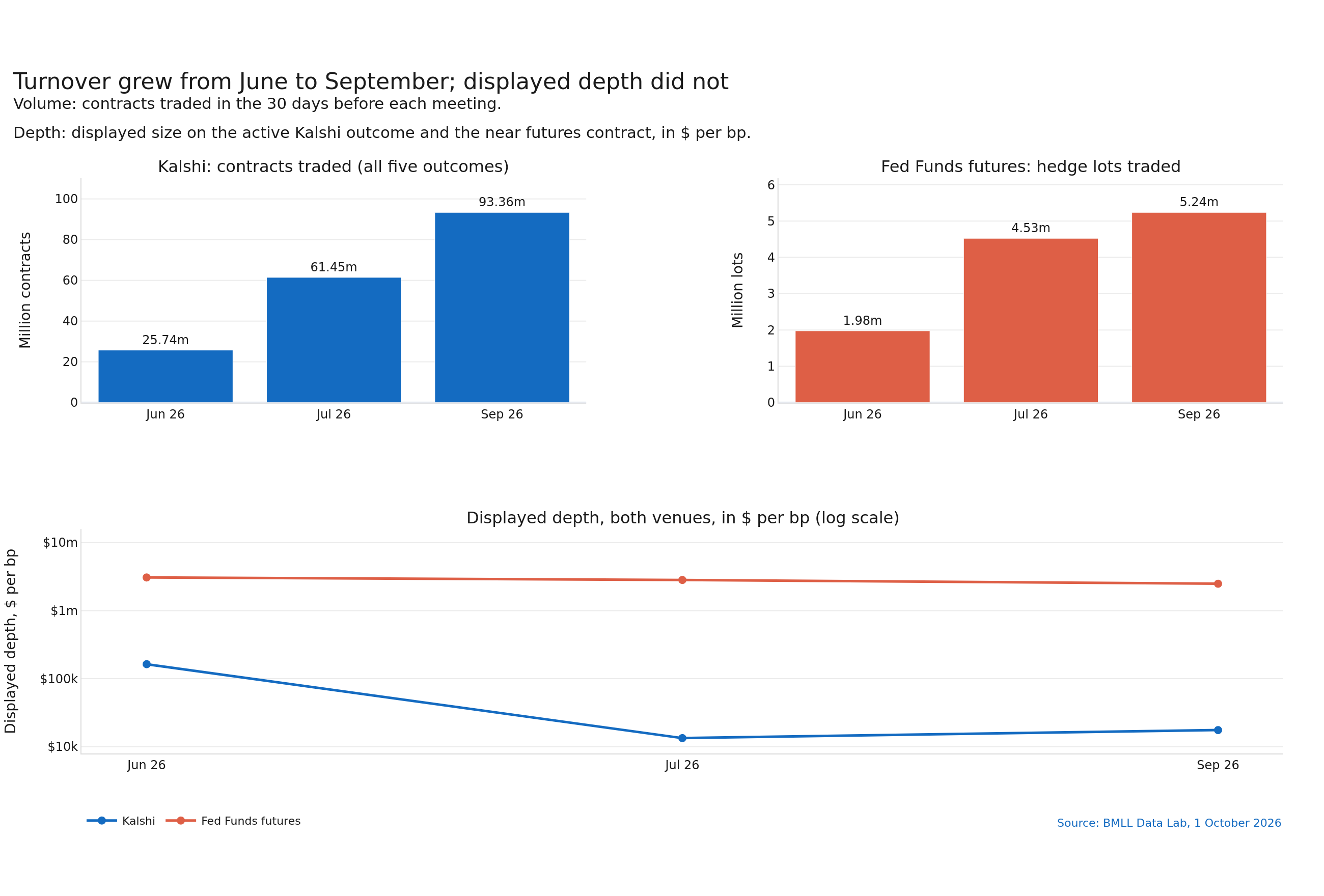
Turnover on Kalshi has grown quickly. As it grows, divergences between CME Fed Funds futures and Kalshi will matter more, because they can present arbitrage opportunities and show different sets of traders setting prices. In this section we compare turnover and displayed depth on the two venues. In the 30 days before each meeting, Kalshi traded 25.74 million contracts in June, 61.45 million in July and 93.36 million in September: September was 52% above July and 3.6 times June, as shown in Figure 5. Over the same windows the Fed Funds futures hedge contracts traded 1.98 million lots, 4.53 million and 5.24 million.

Using Level 2 data and converting displayed size to the common $ per basis point scale (DV01), we can also compare depth of book. Depth on the futures is far larger than on Kalshi: about $2.5 million per bp in September against about $17,500 on Kalshi, a ratio of roughly 140 to 1. Kalshi depth grew from $13,000 in July to $17,500 September, while futures depth eased from $3.1 million to $2.5 million, as seen in Figure 5.

Fig 5: Volumes (contracts traded in the 30 days before each meeting) and displayed depth for Fed Funds futures and Kalshi Fed decision markets

Could the fair-value divergences easily be traded?

For market participants, the most important question is whether these differences between contracts translate into a trading or hedging strategy. In this section, we construct a simple toy strategy to show how these contracts could be traded, for both a passive and aggressive strategy. Our simple execution strategy reduces the Kalshi distribution to the dominant adjacent pair around the market’s main uncertainty, hedges its local rate sensitivity with ZQ contracts, and then tests whether the fair-value edge could be traded against displayed quantities in the respective books.

To create this toy strategy, we first look at five-minute market states where the edge after costs and reserves clears 0.25 cents per Kalshi contract. We then screen these states for situations where a hedge can be built on the Fed Funds futures (1 CME contract is a lot larger than a Kalshi contract). The strategy takes the first position in the study window that passes these filters and carries it until just after the FOMC decision.

Our proposed aggressive strategy crosses both the Kalshi book and the relevant Fed Funds futures book. Our proposed market-making strategy is supposed, unrealistically, to get filled passively, that is without crossing the book. Meeting-to-meeting differences are large:

Meeting sample	Five-minute states with a tradable pair	Kalshi maker / futures taker	Both taker	Futures maker / Kalshi taker
June 2026	4,768	0.0%	0.0%	<0.1% (1 state)
July 2026	5,679	68.1%	52.5%	66.9%
September 2026	5,749	13.2%	1.1%	10.5%

Each percentage is the share of five-minute states, among those where the Kalshi pair test found a tradable pair of adjacent outcomes, in which at least one tested size and direction cleared our threshold of 0.25 cents of net edge per Kalshi contract. That threshold is the dotted line in Fig 6 below. These are not win rates: successive states can describe the same persistent gap and reuse the same displayed liquidity, so they cannot be added into cumulative returns.

Taking liquidity on both venues cleared the threshold in 52.5% of July states but in only 1.1% of September states (64 of 5,749). The maker variants cleared it far more often in both months.

June produced almost no opportunity. Kalshi priced a hold as close to certain (its daily expected decision stayed between -1.0bp and 0), so the hold outcome cost about 96 cents and the other side of the pair only a few cents, leaving nothing to capture after our modelled costs. One five-minute state, on 29 May, cleared the threshold.

July and September were genuine two-way meetings without the same issue. June’s median daily gap was also smaller, 0.79bp against 2.88bp in July. 0.79bp is worth 3.2 cents a contract (1bp is worth 4 cents). In the qualifying both-taker states, costs and reserves took a median 7.8 cents per contract in July, against a median gross edge of 8.4 cents, and 9.1 cents in September, against 9.6 cents. July’s qualifying both-taker states had a median largest tested size of roughly 75,000 Kalshi contracts and a median net edge of 0.69 cents per contract. September’s 64 qualifying both-taker states had a median largest tested size of roughly 7,200 contracts and a median net edge of 0.42 cents. The passive cases look better because assuming passive fills improves entry prices; they also require a fill that the screen does not prove occurred.

Fig 6: Executable-price screen under three execution assumptions: edge after costs and reserves (left) and largest qualifying size (right), one point per 30-minute window.

What would carrying both legs of the trade to the FOMC decision yield?

Our toy strategy is limited by design. It takes the first qualifying pre-decision state for each meeting and execution mode, fixes the quantity and direction at that point, and follows that same hedged position through to the FOMC decision. The P&L numbers below include no optimisation of entry, size or exit, that a real trading strategy would industrialise.

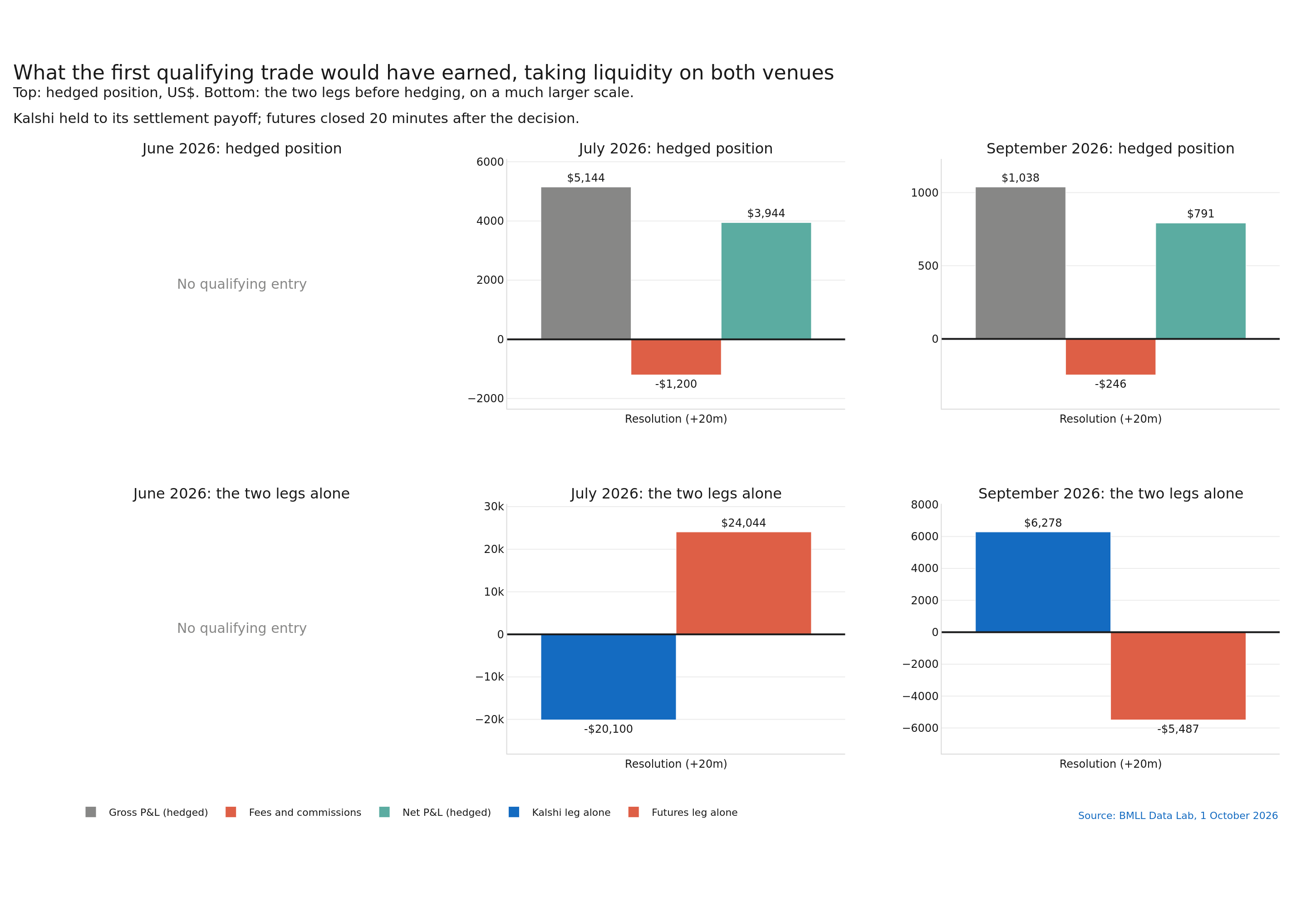
For the first qualifying both-taker entry, July used 86,085 Kalshi contracts, entered on 29 June at the start of the window. At resolution the Kalshi leg was down about US$20,100 net and the futures hedge up about US$24,044, leaving a combined modelled gain of US$3,944 after US$1,200 of fees. In September the first qualifying both-taker entry came on 30 August with 12,493 contracts, and the signs reversed: Kalshi gained about US$6,278 while the futures hedge lost about US$5,487, leaving US$791 after US$246 of fees. The two legs are large and directional, while the combined result is the basis left between them.

The Kalshi-maker entries produce larger counterfactual gains, but only under a full-fill assumption. That version produced modelled resolution P&L of US$8,327 in July and US$3,284 in September (48,011 contracts, entered on 17 August); the futures-maker variant produced US$5,673 and US$566. The single qualifying June state, a futures-maker entry on 29 May, produced US$289.

Further and more realistic simulations would, by design, exhibit greater profitability at scale.

Fig 7: P&L at resolution for the first qualifying both-taker entry: hedged position (top) and the two legs alone (bottom).

The importance of prediction markets data

Prediction markets continue to grow, moving away from sports and digital assets into more traditional factors. For market participants, understanding how these markets behave, and whether they can be used for either hedging or trading is essential.

By utilising the BMLL Data Lab, and its consistent, easy to use multi-asset historical data, we can easily compare Kalshi Fed rate predictions to CME 30-Day Fed futures. We see that there are differences in predicted rate change, reaction speed and liquidity profile, allowing you to quickly start to build simple hedging and trading strategies.

For anyone trading these markets, understanding the relationship between prediction markets and traditional asset classes is now critical to finding new alpha, hedging effectively and managing risk.

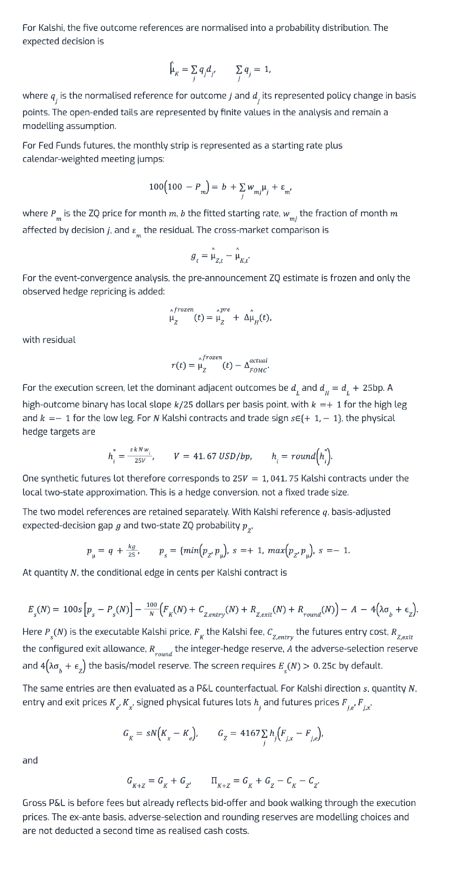
Appendix A: Model, hedge and P&L equations

Sources

Federal Reserve, FOMC calendars and statements: https://www.federalreserve.gov/monetarypolicy/fomccalendars.htm

Federal Reserve, FOMC statement, 29 July 2026: https://www.federalreserve.gov/newsevents/pressreleases/monetary20260729a.htm

Federal Reserve, FOMC statement, 16 September 2026: https://www.federalreserve.gov/newsevents/pressreleases/monetary20260916a.htm

New York Fed, effective federal funds rate methodology: https://www.newyorkfed.org/markets/reference-rates/effr

Kuttner, K., Monetary Policy Surprises and Interest Rates, New York Fed Staff Report 99: https://www.newyorkfed.org/research/staff_reports/sr99.html

CME Group, FedWatch methodology: https://www.cmegroup.com/articles/2023/understanding-the-cme-group-fedwatch-tool-methodology.html

CME Group, 30-Day Federal Funds futures contract rules: https://www.cmegroup.com/rulebook/CBOT/III/22.pdf

Kalshi, fee schedule: https://kalshi.com/docs/kalshi-fee-schedule.pdf

US Bureau of Labor Statistics, CPI release calendar: https://www.bls.gov/schedule/news_release/cpi.htm

Data: BMLL harmonised Level 1, 2 and 3 market data for Kalshi (KLSH) and CME (XCBT), accessed through BMLL Data Lab. Analysis run 1 October 2026.